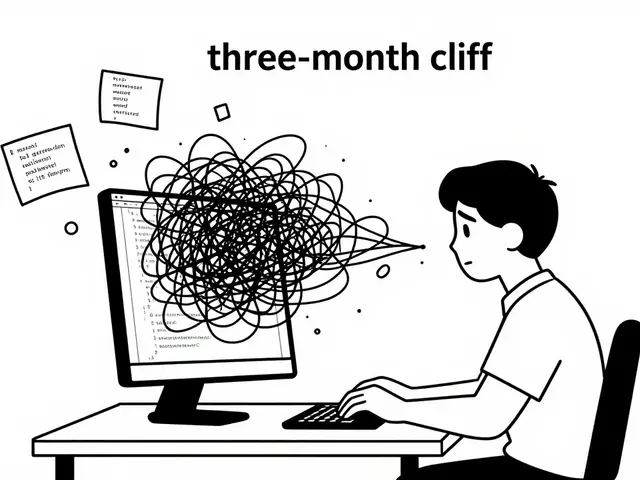
You’re burning cash on GPUs while your LLM sits idle. It sounds counterintuitive, but during standard large language model (LLM) inference, up to 75% of your expensive hardware capacity often goes unused. This isn’t a bug; it’s a feature of how transformers work. They generate text one token at a time, meaning some requests finish quickly while others drag on for seconds. If you schedule them poorly, fast requests wait for slow ones, and your $30,000 NVIDIA H100s spend most of their time doing nothing.
The solution lies in LLM scheduling. This isn’t just about queueing jobs; it’s about dynamically allocating computational resources to match the unpredictable nature of autoregressive generation. Recent benchmarks show that smart scheduling can cut costs by nearly 87% and boost throughput by 3.7x compared to naive approaches. Whether you are running a startup demo or a Fortune 500 enterprise service, getting this right is the difference between profitability and bankruptcy.
The Core Problem: Why Standard Batching Fails
Traditional deep learning models, like image classifiers, have fixed input and output sizes. You can batch them easily because every item takes roughly the same amount of time. LLMs break this rule. They are variable-length, stateful, and memory-intensive. When you use static batching-where you wait for a full batch of requests before starting-the system stalls. A request that needs only 10 tokens blocks a batch waiting for another request that needs 500 tokens.
This inefficiency creates two major bottlenecks:
- Memory Fragmentation: The Key-Value (KV) cache, which stores attention states, gets fragmented. You might have enough total memory, but not in contiguous blocks, leading to out-of-memory errors even when VRAM looks half-full.
- Compute Starvation: GPUs are designed for parallelism. If they are waiting for the longest sequence in a batch to finish, they sit idle instead of processing new incoming requests.
Dr. Jane Chen, a Senior Research Scientist at NVIDIA, noted in 2025 that without sophisticated scheduling, this mismatch leaves the majority of GPU capacity idle. To fix this, we need strategies that treat each token generation step as a schedulable unit, not just the entire request.
Continuous Batching: The Foundation of Modern Serving
The first major shift in LLM serving was moving from static to continuous batching. Systems like vLLM an open-source library for high-throughput and memory-efficient LLM inference and serving popularized this approach. Instead of waiting for a batch to fill, continuous batching adds new requests to the running batch as soon as older ones finish.
Think of it like a restaurant table. In static batching, you seat four people, take orders, cook, serve, and clear the table before seating the next group. If one person orders a steak and another orders soup, the soup eater waits for the steak. Continuous batching lets you seat new customers at empty seats immediately. As soon as the soup finishes, that seat opens up for a new order.
Technically, this requires managing the KV cache dynamically. vLLM uses a technique called PagedAttention, inspired by OS virtual memory paging. It breaks the KV cache into small blocks, allowing non-contiguous storage. This reduces memory fragmentation by over 40%, enabling higher batch sizes and better GPU utilization. According to NVIDIA’s 2024 benchmarks, this alone can push GPU utilization from a dismal 30-40% to a healthy 70-85%.

Predictive Scheduling: Knowing Before You Generate
Continuous batching helps, but it doesn’t solve everything. If you mix very long and very short requests, you still suffer from head-of-line blocking. The best way to mitigate this is prediction. If you know how many tokens a request will likely generate, you can group similar requests together.
Research by Zheng et al. (2023) demonstrated that using lightweight predictors to estimate output lengths can reduce padding waste by 22.3%. These predictors don’t need to be perfect. Even a rough estimate allows the scheduler to bin requests into groups (e.g., 0-50 tokens, 50-100 tokens). By keeping batches homogeneous, you minimize the time faster requests wait for slower ones.
However, predictions aren’t free. Overly complex models add latency. The sweet spot, identified by Agrawal et al. (2023), involves balancing the token budget. Larger budgets (2048 tokens) improve prefill speed, while moderate budgets (512 tokens) optimize end-to-end latency. Advanced systems like Sarathi-Serve a scheduling framework that separates prefill and decode phases to maximize throughput take this further by chunking prefill operations, ensuring that long inputs don’t block ongoing decode steps.
Hierarchical and Workload-Aware Strategies
Not all requests are equal. Some users need sub-100ms responses; others can wait seconds. Hierarchical scheduling prioritizes traffic based on Service Level Objectives (SLOs). Clarifai’s March 2025 benchmark showed that hierarchical policies achieved 99.9th percentile latencies of 87ms, compared to 214ms for simple First-In-First-Out (FIFO) queues.
This approach works best in multi-tenant environments where different clients pay for different tiers. You can implement priority queues where high-priority requests preempt lower-priority ones if resources are tight. But beware: aggressive preemption can cause thrashing. If you constantly interrupt long-running jobs for short bursts, you lose efficiency.
Another emerging trend is workload-aware allocation. Systems like ExeGPT use round-robin or dynamic allocation across layers and blocks. Oh et al. (2024) reported that this method achieves 18.7% higher throughput under strict latency constraints compared to uniform scheduling. It recognizes that different parts of the transformer architecture have different computational demands and schedules accordingly.
Hardware and Memory Optimization Synergies
Scheduling doesn’t exist in a vacuum. It interacts tightly with hardware capabilities. For instance, prefix caching detects repeated contexts. If multiple users ask questions about the same document, llm-d can reuse the computed KV cache for that prefix. Red Hat’s case study showed this reduces time-to-first-token by 63.4ms on average, with detection accuracy hitting 98.7%.
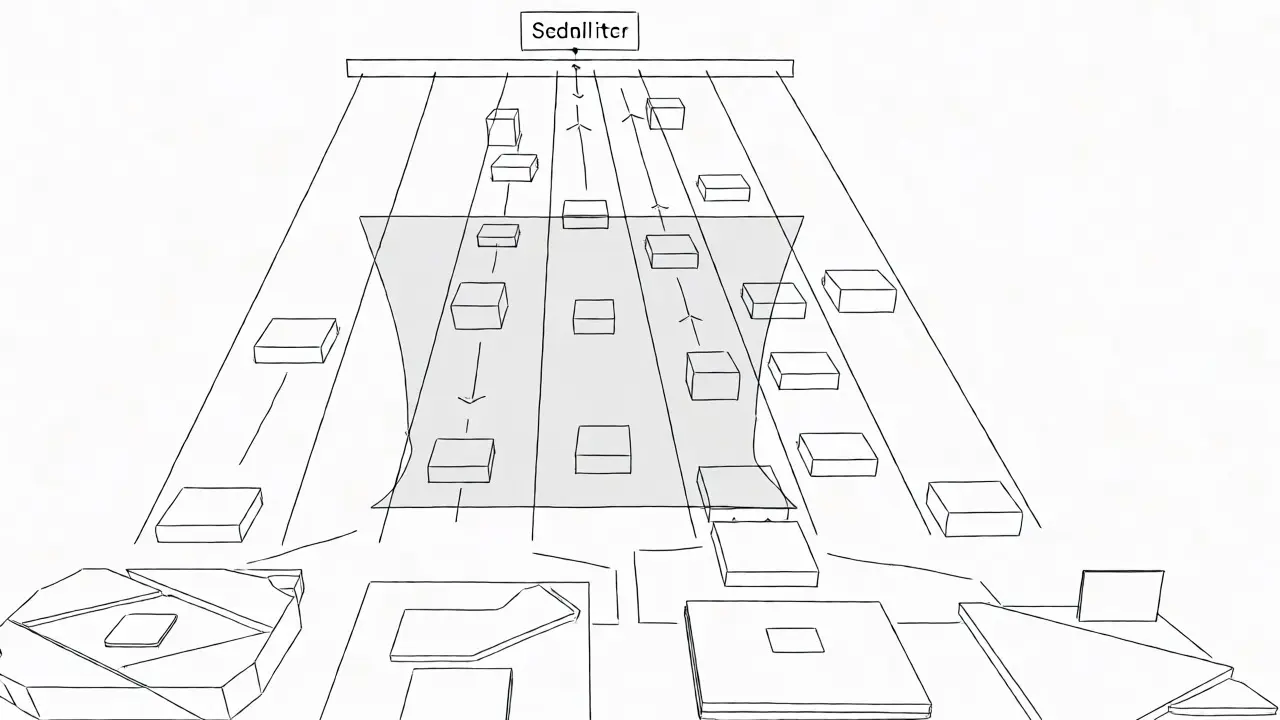
Furthermore, heterogeneous clusters require specialized handling. Not all GPUs are identical. Mixing A100s and H100s means varying memory bandwidth and compute power. NVIDIA’s Triton Inference Server 3.0 introduced hardware-aware scheduling that routes requests to the most suitable GPU type. This prevents powerful H100s from being bottlenecked by memory-bound tasks that could run fine on cheaper A100s.
| Strategy | Key Mechanism | Throughput Gain | Implementation Effort | Best Use Case |
|---|---|---|---|---|
| Static Batching | Fixed batch intervals | Baseline (1.0x) | Low | Offline processing, predictable loads |
| Continuous Batching (vLLM) | In-flight request insertion + PagedAttention | 2.1x - 3.4x | Moderate (2-3 weeks) | General production serving |
| Predictive Scheduling (Sarathi) | Output length estimation + Chunked Prefill | 4.7x - 5.9x | High (6-8 weeks) | High-concurrency, mixed workloads |
| Hierarchical Priority | SLO-based queuing | Variable (Latency focus) | Moderate | Multi-tenant SaaS with tiered pricing |
Implementation Pitfalls and Best Practices
Adopting these strategies isn’t plug-and-play. One common failure mode is inaccurate length prediction. Zheng et al. warned that poor predictions can cause an 18-22% throughput loss. Mitigation involves ensemble models or adaptive bounds. Chen et al. (2025) proposed initializing with lower prediction bounds and adjusting dynamically, yielding 15.8% higher utilization than conservative static bounds.
Another trap is overhead. Complex schedulers add milliseconds per request. AWS Principal Engineer Mark Thompson cautioned that overly complex logic can introduce 15-20ms of overhead, negating benefits for applications requiring sub-200ms latency. Always profile your scheduler. If your inference takes 50ms, adding a 10ms scheduler decision loop is a 20% penalty.
Start simple. Deploy vLLM with continuous batching first. Measure your utilization. If you’re still below 70%, look into predictive scheduling. Only move to hierarchical or distributed frameworks like llm-d if you have specific multi-tenant or cross-cluster requirements. Remember, Gartner predicts that by 2026, 85% of enterprise deployments will use specialized scheduling, so building this expertise now future-proofs your infrastructure.
What is the main benefit of continuous batching over static batching?
Continuous batching eliminates the wait time for fixed batch intervals. It allows new requests to enter the processing queue as soon as previous ones complete, significantly increasing GPU utilization from typically 30-40% to 70-85% by reducing idle time caused by variable-length outputs.
How does PagedAttention improve LLM serving?
PagedAttention, used in vLLM, manages the KV cache in non-contiguous memory blocks, similar to virtual memory in operating systems. This reduces memory fragmentation by over 40%, allowing larger batch sizes and preventing out-of-memory errors despite variable sequence lengths.
Do I need predictive scheduling for my LLM application?
You should consider predictive scheduling if you handle high concurrency (500+ concurrent requests) or have highly variable output lengths. While it adds engineering complexity (6-8 weeks implementation), it can deliver 4.7-5.9x throughput gains by grouping similar requests and minimizing padding waste.
What hardware is recommended for optimized LLM scheduling?
Production deployments typically require NVIDIA A100 or H100 GPUs with at least 40GB VRAM. These cards offer the memory bandwidth and tensor core performance necessary to leverage advanced scheduling techniques like chunked prefill and paged attention effectively.
Can scheduling help reduce operational costs?
Yes, significantly. Optimized resource utilization through advanced scheduling has been shown to reduce operational costs by up to 86.92% in benchmark studies. By maximizing throughput per GPU, you can serve more requests with fewer instances, directly lowering cloud spending.
 Artificial Intelligence